How To Create A Set In Python 3

This series will innovate you to graphing in python with Matplotlib, which is arguably the almost popular graphing and data visualization library for Python.
Installation
The easiest way to install matplotlib is to use pip. Blazon following command in final:

pip install matplotlib

OR, you can download it from here and install it manually.

Getting started ( Plotting a line)

Python

              import              matplotlib.pyplot equally plt            
              ten                            =              [              one              ,              2              ,              3              ]            
              y                            =              [              2              ,              4              ,              1              ]            
              plt.plot(x, y)            
              plt.xlabel(              'x - centrality'              )            
              plt.ylabel(              'y - axis'              )            
              plt.title(              'My kickoff graph!'              )            
              plt.show()            

Output:

mp1

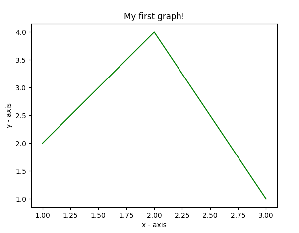
The code seems cocky-explanatory. Following steps were followed:

Ascertain the 10-centrality and respective y-axis values as lists.
Plot them on canvass using .plot() function.
Give a proper noun to 10-centrality and y-centrality using .xlabel() and .ylabel() functions.
Give a title to your plot using .championship() function.
Finally, to view your plot, nosotros use .show() office.

Plotting two or more lines on aforementioned plot

Python

              import              matplotlib.pyplot as plt            
              x1                            =              [              1              ,              2              ,              three              ]            
              y1                            =              [              two              ,              4              ,              1              ]            
              plt.plot(x1, y1, label                            =              "line 1"              )            
              x2                            =              [              1              ,              2              ,              3              ]            
              y2                            =              [              iv              ,              one              ,              3              ]            
              plt.plot(x2, y2, characterization                            =              "line 2"              )            
              plt.xlabel(              'ten - axis'              )            
              plt.ylabel(              'y - centrality'              )            
              plt.championship(              'Two lines on same graph!'              )            
              plt.legend()            
              plt.show()            

Output:

mp2

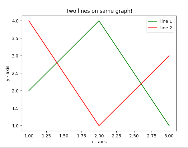
Here, we plot 2 lines on the same graph. We differentiate betwixt them past giving them a name(label) which is passed every bit an argument of the .plot() office.
The minor rectangular box giving information about the type of line and its colour is called a legend. We tin can add a fable to our plot using .fable() office.

Customization of Plots

Hither, nosotros discuss some elementary customizations applicable to almost whatever plot.

Python

              import              matplotlib.pyplot as plt            
              10                            =              [              1              ,              2              ,              3              ,              four              ,              v              ,              6              ]            
              y                            =              [              two              ,              4              ,              1              ,              5              ,              2              ,              6              ]            
              plt.plot(x, y, colour              =              'green'              , linestyle              =              'dashed'              , linewidth                            =              three              ,            
                            mark              =              'o'              , markerfacecolor              =              'blue'              , markersize              =              12              )            
              plt.ylim(              1              ,              8              )            
              plt.xlim(              i              ,              8              )            
              plt.xlabel(              'x - axis'              )            
              plt.ylabel(              'y - centrality'              )            
              plt.title(              'Some absurd customizations!'              )            
              plt.show()            

Output:

mp3

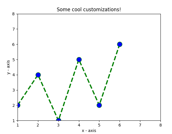
Every bit you can run into, nosotros accept done several customizations like

setting the line-width, line-style, line-color.
setting the marker, marker'southward face colour, marker'south size.
overriding the 10 and y-axis range. If overriding is not done, pyplot module uses the machine-calibration feature to set the axis range and scale.

Bar Chart

Python

              import              matplotlib.pyplot as plt            
              left                            =              [              1              ,                            2              ,                            3              ,                            iv              ,                            5              ]            
              acme                            =              [              ten              ,                            24              ,                            36              ,                            40              ,                            5              ]            
              tick_label                            =              [              'one'              ,                            '2'              ,                            'three'              ,                            'iv'              ,                            'five'              ]            
              plt.bar(left, acme, tick_label                            =              tick_label,            
                            width                            =              0.8              , colour                            =              [              'red'              ,                            'green'              ])            
              plt.xlabel(              'x - axis'              )            
              plt.ylabel(              'y - axis'              )            
              plt.title(              'My bar chart!'              )            
              plt.show()            

Output :

mp4

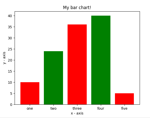
Hither, we use plt.bar() function to plot a bar chart.
x-coordinates of the left side of bars are passed forth with the heights of bars.
yous can besides requite some names to 10-axis coordinates past defining tick_labels

Histogram

Python

              import              matplotlib.pyplot as plt            
              ages                            =              [              2              ,              5              ,              70              ,              40              ,              30              ,              45              ,              fifty              ,              45              ,              43              ,              40              ,              44              ,            
                            60              ,              7              ,              13              ,              57              ,              xviii              ,              90              ,              77              ,              32              ,              21              ,              20              ,              40              ]            
              range              =              (              0              ,                            100              )            
              bins                            =              10
              plt.hist(ages, bins,                            range              , color                            =              'dark-green'              ,            
                            histtype                            =              'bar'              , rwidth                            =              0.8              )            
              plt.xlabel(              'age'              )            
              plt.ylabel(              'No. of people'              )            
              plt.title(              'My histogram'              )            
              plt.show()            

Output:

mp5

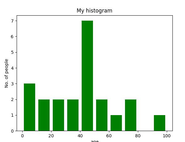
Here, we use plt.hist() function to plot a histogram.
frequencies are passed as the ages list.
The range could be set past defining a tuple containing min and max values.
The next step is to "bin" the range of values—that is, divide the entire range of values into a series of intervals—and then count how many values fall into each interval. Here we have divers bins = x. So, there are a total of 100/10 = 10 intervals.

Scatter plot

Python

              import              matplotlib.pyplot every bit plt            
              x                            =              [              ane              ,              two              ,              3              ,              4              ,              5              ,              6              ,              seven              ,              8              ,              nine              ,              10              ]            
              y                            =              [              2              ,              four              ,              5              ,              7              ,              6              ,              viii              ,              nine              ,              11              ,              12              ,              12              ]            
              plt.scatter(x, y, label              =              "stars"              , color              =              "green"              ,            
                            marker              =              "*"              , due south              =              30              )            
              plt.xlabel(              '10 - axis'              )            
              plt.ylabel(              'y - axis'              )            
              plt.championship(              'My besprinkle plot!'              )            
              plt.legend()            
              plt.show()            

Output:

mp6

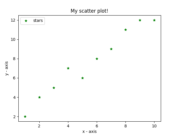
Here, we use plt.scatter() function to plot a besprinkle plot.
As a line, we define x and corresponding y-axis values here too.
marker argument is used to set the graphic symbol to utilize as a marking. Its size can be defined using the s parameter.

Pie-chart

Python

              import              matplotlib.pyplot every bit plt            
              activities                            =              [              'eat'              ,                            'slumber'              ,                            'piece of work'              ,                            'play'              ]            
              slices                            =              [              iii              ,                            seven              ,                            8              ,                            6              ]            
              colors                            =              [              'r'              ,                            'y'              ,                            'g'              ,                            'b'              ]            
              plt.pie(slices, labels                            =              activities, colors              =              colors,            
                            startangle              =              xc              , shadow                            =              Truthful              , explode                            =              (              0              ,                            0              ,                            0.1              ,                            0              ),            
                            radius                            =              i.2              , autopct                            =              '%1.1f%%'              )            
              plt.legend()            
              plt.show()            

The output of in a higher place program looks like this:

mp7

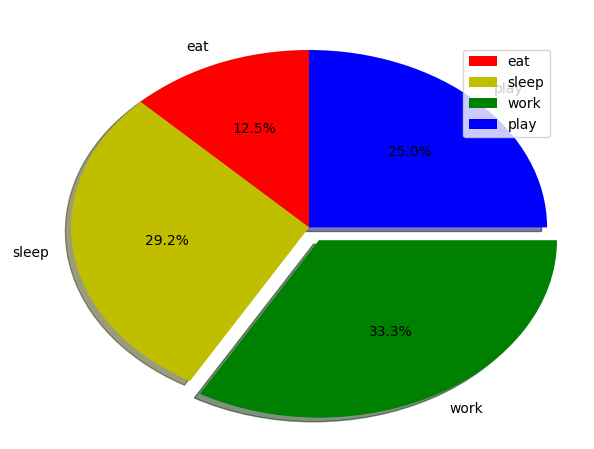
Here, nosotros plot a pie chart by using plt.pie() method.
Beginning of all, nosotros define the labels using a listing chosen activities.
Then, a portion of each label tin be defined using another listing called slices.
Colour for each label is defined using a list called colors.
shadow = True will bear witness a shadow beneath each label in pie chart.
startangle rotates the start of the pie chart by given degrees counterclockwise from the x-axis.
explode is used to ready the fraction of radius with which nosotros beginning each wedge.
autopct is used to format the value of each label. Here, we have set information technology to show the percent value simply upto 1 decimal identify.

Plotting curves of given equation

Python

              import              matplotlib.pyplot as plt            
              import              numpy as np            
              ten                            =              np.arange(              0              ,                            2              *              (np.pi),                            0.1              )            
              y                            =              np.sin(x)            
              plt.plot(x, y)            
              plt.show()            

The output

of above program looks like this:

mp8

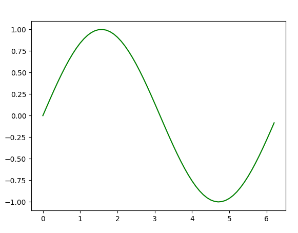
Here, nosotros apply NumPy which is a general-purpose assortment-processing package in python.

To set up the ten-axis values, nosotros use the np.arange() method in which the showtime 2 arguments are for range and the third one for step-wise increment. The result is a NumPy array.
To get corresponding y-axis values, we simply use the predefined np.sin() method on the NumPy array.
Finally, we plot the points by passing x and y arrays to the plt.plot() role.

So, in this office, nosotros discussed various types of plots nosotros tin create in matplotlib. There are more plots that haven't been covered simply the most meaning ones are discussed here –

Graph Plotting in Python | Prepare 2
Graph Plotting in Python | Set 3

This article is contributed by Nikhil Kumar. If you similar GeeksforGeeks and would like to contribute, you tin also write an commodity using write.geeksforgeeks.org or mail your commodity to review-team@geeksforgeeks.org. See your article appearing on the GeeksforGeeks main page and aid other Geeks.
Please write comments if you find annihilation wrong, or you want to share more information about the topic discussed above.